The Shelter Wedge: How Housing Supply Constraints Amplify the Great Decompression

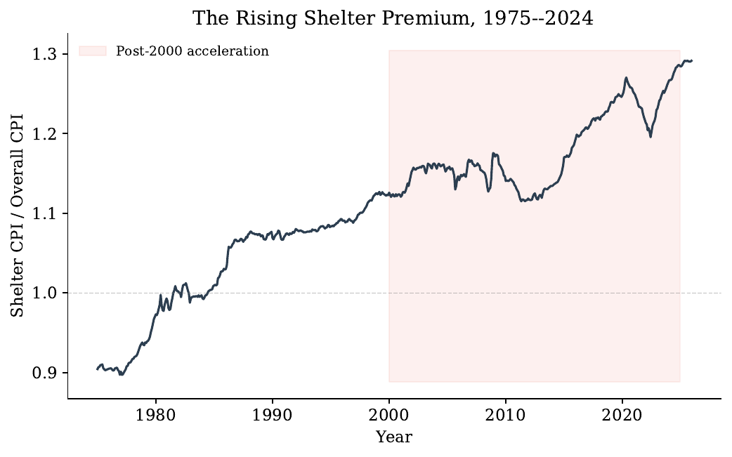
Since 1970, shelter costs in the United States have grown 44% faster than overall prices. The ratio of shelter CPI to overall CPI stood at 0.897 in 1970; by 2025 it had climbed to 1.291. Housing is not just another line item that inflated with everything else. It has persistently outpaced the rest of the consumption basket for five decades, and it absorbs 30 to 40% of income for median earners. This companion essay walks through what that gap means, why a supply-constrained housing market should amplify it, and why the state-level test in the paper comes back null.

The shelter wedge

Income inequality is usually measured in nominal terms: the ratio of 80th-percentile to median household income, top-decile income shares, skill premia. But households consume goods and services, not nominal income, and housing occupies a singular position among those expenditures. If shelter costs rise faster for the households that devote the largest share of income to rent and mortgage payments, even modest nominal divergence translates into large differences in material living standards.

We call this mechanism the shelter wedge: the amplification of nominal income inequality through differential shelter cost inflation. The wedge should be largest where housing supply cannot respond. When supply is inelastic, because of geography, zoning, or regulation, rising incomes at the top of the distribution are capitalized into prices rather than absorbed by construction. High earners bid for a fixed stock of desirable housing, and middle-income households competing in the same local market pay the price.

What the model predicts

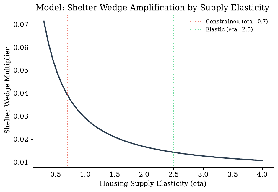
A two-neighborhood spatial sorting model makes the intuition precise. Its key output is the shelter wedge multiplier: how much the gap in shelter burdens widens when the income ratio between high and middle earners rises. The multiplier falls sharply as housing supply elasticity rises.

Calibrated to observed rent burdens, a constrained market (elasticity 0.7) amplifies the wedge by a factor of 2.2 relative to an elastic market (elasticity 2.5). In the model's counterfactual, the same income divergence raises the shelter burden gap by 6.9 percentage points in constrained markets against 3.1 points in elastic ones. That is a strong, testable prediction: places that cannot build should show rent burdens diverging as national income inequality widens.

What the data say

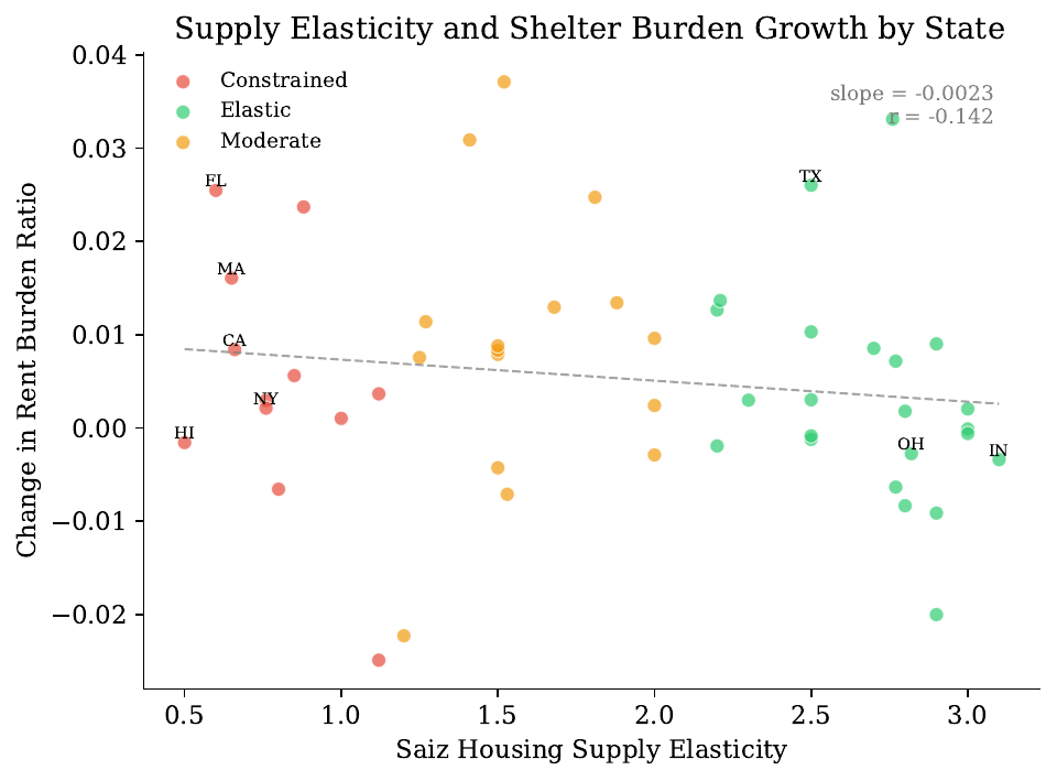
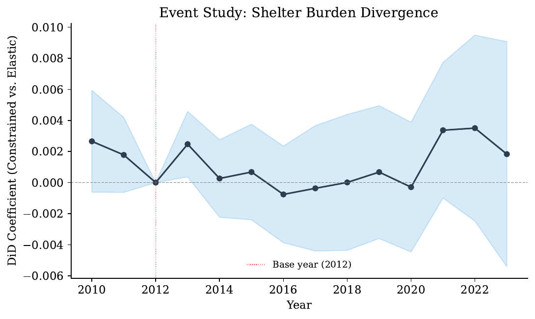
The paper tests the prediction on a panel of 714 state-year observations covering 51 states (including the District of Columbia) from 2010 to 2023, using the Saiz (2010) housing supply elasticities to classify 12 states as supply-constrained and 23 as elastic. The difference-in-differences design asks whether rent burdens in constrained states pulled away from elastic states as the national 80th-to-50th income ratio rose.

They did not.

The baseline estimate of the shelter wedge amplifier is 0.0107 with a standard error of 0.0845 (p = 0.899). Adding economic controls flips the sign without adding significance. Permutation inference across 1,000 random reassignments of treatment yields p = 0.868. The event study shows no pre-trends, and no post-treatment divergence either.

National local projections push in the same direction: the shelter CPI response to income shocks has weakened since 2000, with the 12-month cumulative response falling from 0.0182 before 2000 to 0.0027 after. Whatever is driving the shelter premium's post-2000 acceleration, it is not showing up as a state-level supply-constraint interaction.

Why a null is informative

A precisely estimated null at the state level does not mean the mechanism is absent. It means the state is the wrong unit of analysis. The sorting processes that drive housing cost inflation are local: high-income households bidding up prices in particular neighborhoods of particular metros. California contains both San Francisco, one of the most constrained markets in the country, and the comparatively elastic Inland Empire; averaging them into one observation buries exactly the variation the theory is about. Two caveats sharpen the point. The design’s minimum detectable effect is large (about 124% of the mean rent burden), so only a very big state-level wedge could have been found. And the one specification using state-specific rather than national income gaps comes back marginally significant (p = 0.059), hinting that the mechanism surfaces as soon as the income variation gets more local.

That reading is consistent with the metro-level literature: Hsieh and Moretti’s estimate that housing constraints in high-productivity cities cost the U.S. decades of aggregate growth, and Diamond’s evidence on skill sorting within metros. The shelter wedge is real in the aggregate time series; it just lives below the state.

Where this goes next

The natural sequel is the same design at the metropolitan or neighborhood level, where both the income variation and the supply constraints are measured where the bidding actually happens. As income divergence continues and supply stays tight in high-productivity cities, the shelter wedge remains a candidate for the main channel through which nominal inequality becomes lived inequality. The full model, data construction, identification assumptions, and robustness battery are in the paper.